DECISION TREE ( 의사 결정 트리 )

Decision Tree ?

 

데이터를 나무 구조로 도표화하여 분류 및 회귀를 수행하는 머신러닝 알고리즘

 

* 일종의 스무고개 

* 특정 기준에 대한 정답/오답에 따라 대상의 범위를 좁혀나감

* 분류(DecisionTreeClassifier)와 회귀(DecisionTreeRegressor)가 모두 가능 + 다중출력 작업까지

* 데이터 전처리 불필요 -> scaling 불필요

 

1️⃣ 간단한 시각화

from sklearn.datasets import load_iris
from sklearn.tree import DecisionTreeClassifier
import numpy as np
import pandas as pd
iris = load_iris() # 붓꽃데이터 로드
iris.keys() # iris 데이터 확인

X = iris.data[:, 2:] # petal length & petal width
y = iris.target

tree = DecisionTreeClassifier(max_depth = 2) # max_depth : 결정나무의 깊이 즉 가지갈래의 개수라고 생각하면 쉬움
tree.fit(X,y)

from sklearn.tree import plot_tree
import matplotlib.pyplot as plt
plt.figure(figsize = (10,10))
plot_tree(tree,
         feature_names = iris.feature_names[2:],
         class_names = iris.target_names,
         filled = True, # filled : 분류에 따라 색칠
         rounded = True # rounded : 박스 모서리 둥글게
         )

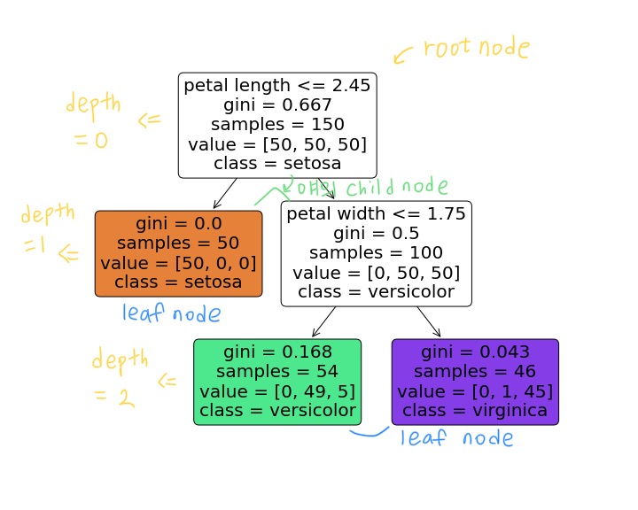
* root node / child node / leaf node 

* samples : 얼마나 많은 training sample이 적용됐는지

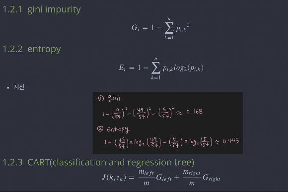
* gini : 불순도(impurity) 측정 => gini impurity가 default이나 criterion = 'entropy'로 설정 가능

 

i번째 노드, k번째 클래스

# 지니 불순도 / 엔트로피 

둘 다 불순도를 측정하는 지표. 한 노드의 모든 샘플들이 같은 클래스로 분류된다면 불순도가 0에 가까워짐( = 순도가 높다 )

-> 즉, 샘플들이 하나의 클래스로 분류가 잘 된다는 의미를 나타내는 척도이므로 최소화시켜야 함

불순도를 무엇으로 지정하든 결정트리의 모양엔 지장이 없으나 entropy가 로그계산으로 인해 gini보다 계산이 느림

혹은 다른 트리가 만들어지는 경우에 지니불순도는 가장 빈도가 높은 클래스를 한쪽 가지에 고립시키고, 엔트로피는 균형있는 트리를 만드는 경향이 있음

 

# CART Algorithm

특성값(ex - petal length)과 임계값(ex - 2.45)을 이용하여 두개의 서브셋으로 나눔 -> '두개'의 subset이므로 child node는 단 2개 => 이진분류

id3 알고리즘을 이용하면 둘 이상의 child node가 있는 트리 생성 가능 

 

from matplotlib.colors import ListedColormap

def plot_decision_boundary(clf, X, y, axes=[0, 7.5, 0, 3], iris=True, legend=False, plot_training=True):
    x1s = np.linspace(axes[0], axes[1], 100)
    x2s = np.linspace(axes[2], axes[3], 100)
    x1, x2 = np.meshgrid(x1s, x2s)
    X_new = np.c_[x1.ravel(), x2.ravel()]
    y_pred = clf.predict(X_new).reshape(x1.shape)
    custom_cmap = ListedColormap(['#fafab0','#9898ff','#a0faa0'])
    plt.contourf(x1, x2, y_pred, alpha=0.3, cmap=custom_cmap)
    if not iris:
        custom_cmap2 = ListedColormap(['#7d7d58','#4c4c7f','#507d50'])
        plt.contour(x1, x2, y_pred, cmap=custom_cmap2, alpha=0.8)
    if plot_training:
        plt.plot(X[:, 0][y==0], X[:, 1][y==0], "yo", label="Iris setosa")
        plt.plot(X[:, 0][y==1], X[:, 1][y==1], "bs", label="Iris versicolor")
        plt.plot(X[:, 0][y==2], X[:, 1][y==2], "g^", label="Iris virginica")
        plt.axis(axes)
    if iris:
        plt.xlabel("Petal length", fontsize=14)
        plt.ylabel("Petal width", fontsize=14)
    else:
        plt.xlabel(r"$x_1$", fontsize=18)
        plt.ylabel(r"$x_2$", fontsize=18, rotation=0)
    if legend:
        plt.legend(loc="lower right", fontsize=14)

plt.figure(figsize=(8, 4))
plot_decision_boundary(tree, X, y)
plt.plot([2.45, 2.45], [0, 3], "k-", linewidth=2)
plt.plot([2.45, 7.5], [1.75, 1.75], "k--", linewidth=2)
plt.text(1.40, 1.0, "Depth=0 \nsetosa", fontsize=15)
plt.text(3.2, 1.4, "virginica \n\n Depth=1 \n\nversicolor", fontsize=13)

 

display(tree.predict_proba([[3.7,2.47]])) # [0/46, 1/46, 45/46]
tree.predict([[3.7,2.47]]) # virginica로 분류

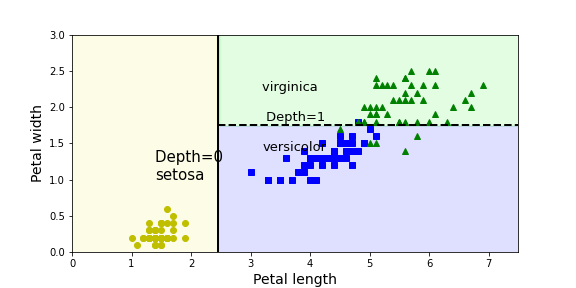
예를 들어 꽃잎 길이 3.7, 꽃잎 너비 2.47인 꽃을 분류하고자 한다면 virginica로 분류될 확률이 높아보임 

predict_proba로 확인 시 virginica로 분류될 확률이 97% => predict로 확인시 array([[2]])(즉, virginica)로 분류되는 것 확인할 수 있다.

 

2️⃣ 규제 매개변수

훈련 전에 파라미터 수가 결정되지 않은 모델 = 비파라미터 모델 -> 과대적합 위험

반면, 훈련 전에 파라미터가 정해진 모델 = 파라미터 모델  -> 과소적합 위험

 

결정트리는 규제가 없어 scale에 자유로움. 따라서 비파라미터모델 -> 과대적합 위험에서 회피하기 위해 매개변수로 모델에 자유도를 제한하는 규제를 함

이렇게 매개변수로 설정해주는 경우는 사전가지치기인데, 비용복잡도에 기반하여 사후가지치기를 하기 위해 ccp_alpha 매개변수가 추가되었다고 함.

또는 카이제곱검정을 통해 (sklearn.feature_selection.chi2) 리프노드 바로 위의 효과없는 노드 삭제하는 가지치기도 가능

 

https://scikit-learn.org/stable/modules/generated/sklearn.tree.DecisionTreeClassifier.html

sklearn.tree.DecisionTreeClassifier — scikit-learn 0.24.2 documentation

DecisionTreeClassifier()

* max_depth : 최대 깊이 제어

* min_samples_split : 노드가 분할되기 위해 가져야 하는 최소 샘플 수 

* min_samples_leaf : leaf node가 가져야하는 최소 샘플 수 

* max_leaf_nodes : leaf node의 최대 개수

* max_features : 각 노드에서 분할에 사용할 최대 특성 수

 

from sklearn.datasets import make_moons
Xm, ym = make_moons(n_samples=100, noise=0.25, random_state=53)

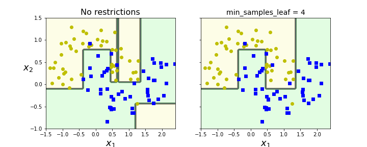
deep_tree_clf1 = DecisionTreeClassifier(random_state=42) # 규제하지 않은 모델
deep_tree_clf2 = DecisionTreeClassifier(min_samples_leaf=4, random_state=42) # min_samples_leaf = 4로 규제를 둔 모델
deep_tree_clf1.fit(Xm, ym)
deep_tree_clf2.fit(Xm, ym)

fig, axes = plt.subplots(ncols=2, figsize=(10, 4), sharey=True)
plt.sca(axes[0])
plot_decision_boundary(deep_tree_clf1, Xm, ym, axes=[-1.5, 2.4, -1, 1.5], iris=False)
plt.title("No restrictions", fontsize=16)
plt.sca(axes[1])
plot_decision_boundary(deep_tree_clf2, Xm, ym, axes=[-1.5, 2.4, -1, 1.5], iris=False)
plt.title("min_samples_leaf = {}".format(deep_tree_clf2.min_samples_leaf), fontsize=14)
plt.ylabel("")

확실히 규제를 둔 오른쪽이 왼쪽보다 일반화가 수월할 것처럼 보인다.

 

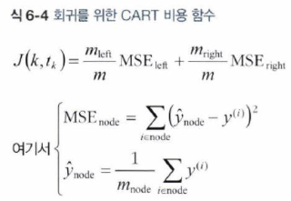
3️⃣ 결정트리 회귀

DecisionTreeRegressor()

* class가 아닌, value를 예측

* MSE를 최소화하는 방향으로 분할해야 함.

* 분류와 마찬가지로 매개변수를 통한 규제로 과대적합 위험을 회피

분류의 경우엔 mse부분이 gini

# 2차식으로 만든 데이터셋 + 잡음
np.random.seed(42)
m = 200
X = np.random.rand(m, 1)
y = 4 * (X - 0.5) ** 2
y = y + np.random.randn(m, 1) / 10

from sklearn.tree import DecisionTreeRegressor

tree_reg = DecisionTreeRegressor(max_depth=2, random_state=42) # 최대 깊이 2로 규제파라미터 설정
tree_reg.fit(X, y)

plt.figure(figsize = (8,8))
plot_tree(tree_reg,
         feature_names = ['x1'],
         rounded = True,
         filled = True)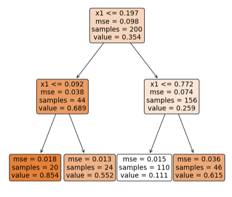

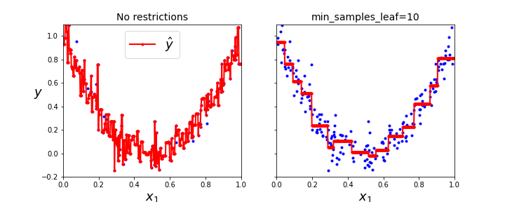
값을 예측하는 DTR. default criterion = 'mse'

tree_reg1 = DecisionTreeRegressor(random_state=42) # 규제 x
tree_reg2 = DecisionTreeRegressor(random_state=42, min_samples_leaf=10) # 규제 o
tree_reg1.fit(X, y)
tree_reg2.fit(X, y)

x1 = np.linspace(0, 1, 500).reshape(-1, 1)
y_pred1 = tree_reg1.predict(x1)
y_pred2 = tree_reg2.predict(x1)

fig, axes = plt.subplots(ncols=2, figsize=(10, 4), sharey=True)

plt.sca(axes[0])
plt.plot(X, y, "b.")
plt.plot(x1, y_pred1, "r.-", linewidth=2, label=r"$\hat{y}$")
plt.axis([0, 1, -0.2, 1.1])
plt.xlabel("$x_1$", fontsize=18)
plt.ylabel("$y$", fontsize=18, rotation=0)
plt.legend(loc="upper center", fontsize=18)
plt.title("No restrictions", fontsize=14)

plt.sca(axes[1])
plt.plot(X, y, "b.")
plt.plot(x1, y_pred2, "r.-", linewidth=2, label=r"$\hat{y}$")
plt.axis([0, 1, -0.2, 1.1])
plt.xlabel("$x_1$", fontsize=18)
plt.title("min_samples_leaf={}".format(tree_reg2.min_samples_leaf), fontsize=14)

규제가 있는 오른쪽이 왼쪽보다 훨씬 일반화가 쉬울 것. 왼쪽은 과대적합된 것으로 보임

4️⃣ 결정 트리의 불안정성

1. 훈련 데이터의 회전에 민감함 -> PCA로 데이터에 맞도록 보정해줌

# 1. 훈련 데이터의 회전

np.random.seed(6)
Xs = np.random.rand(100, 2) - 0.5
ys = (Xs[:, 0] > 0).astype(np.float32) * 2

angle = np.pi / 4
rotation_matrix = np.array([[np.cos(angle), -np.sin(angle)], [np.sin(angle), np.cos(angle)]])
Xsr = Xs.dot(rotation_matrix)

tree_clf_s = DecisionTreeClassifier(random_state=42)
tree_clf_s.fit(Xs, ys)
tree_clf_sr = DecisionTreeClassifier(random_state=42)
tree_clf_sr.fit(Xsr, ys)

fig, axes = plt.subplots(ncols=2, figsize=(10, 4), sharey=True)
plt.sca(axes[0])
plot_decision_boundary(tree_clf_s, Xs, ys, axes=[-0.7, 0.7, -0.7, 0.7], iris=False)
plt.sca(axes[1])
plot_decision_boundary(tree_clf_sr, Xsr, ys, axes=[-0.7, 0.7, -0.7, 0.7], iris=False)
plt.ylabel("")

두 경우 모두 분류는 잘 됐지만, 오른쪽 경우는 구불구불하여 일반화가 쉽지 않음

 

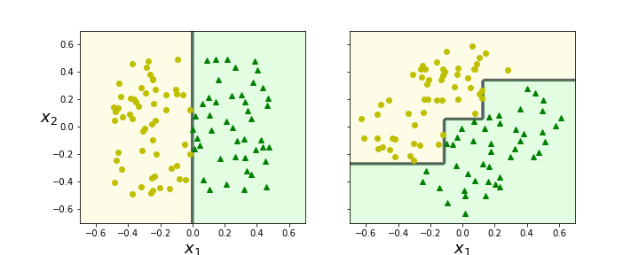
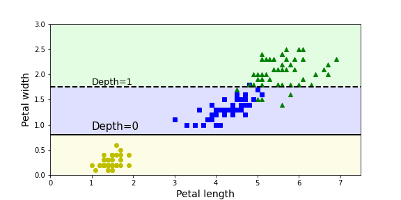
2. 사소한 훈련 데이터 변화에도 민감함 => 이 불안정성을 극복하기 위해 랜덤포레스트 활용

# 2. 사소한 훈련 데이터 변화 -> 규제 매개변수도 동일하지만 아까와 난수 시드 순서만 다르게 함
iris = load_iris()
X = iris.data[:, 2:] # 꽃잎 길이와 너비
y = iris.target

tree_clf_tweaked = DecisionTreeClassifier(max_depth=2, random_state=40)
tree_clf_tweaked.fit(X, y)
plt.figure(figsize=(8, 4))
plot_decision_boundary(tree_clf_tweaked, X, y, legend=False)
plt.plot([0, 7.5], [0.8, 0.8], "k-", linewidth=2)
plt.plot([0, 7.5], [1.75, 1.75], "k--", linewidth=2)
plt.text(1.0, 0.9, "Depth=0", fontsize=15)
plt.text(1.0, 1.80, "Depth=1", fontsize=13)

plt.savefig('image/change.png')

난수 시드 순서만 다르게 했는데 완전히 다른 결과 ・・・ => RandomForest